Score Centering Is a Straight-Through Estimator

Marek and Ryabinin (2026) introduce score centering, an additive correction that stabilises RL on language models when the inference engine that produced the rollouts does not exactly match the trainer that computes the gradients. Their derivation is a covariance identity. Writing \(\bar s\) for the expected score under the sampler, the expected update at a prefix splits as

\[\underbrace{\mathbb{E}_q\!\left[R\, s_{y_t}\right]}_{\text{policy gradient}} = \underbrace{\mathbb{E}_q[R]\, \bar s}_{\text{drift}} + \underbrace{\mathrm{Cov}_q\!\left(R, s_{y_t}\right)}_{\text{signal}},\]

and the drift term — which knows nothing about which rollouts succeeded — is the negative gradient of a cross-entropy loss with the sampler as teacher. Vanilla policy gradient under mismatch is quietly distilling the trainer toward a biased copy of itself, and since that copy is resynced from the trainer every step, the error compounds instead of converging. Score centering subtracts \(\bar s\) and the drift cancels exactly.

I have nothing to correct in that derivation. What I want to add is a name for the object, because the name comes with a literature. The estimator that drift afflicts is a straight-through estimator, and the setting it lives in is quantization-aware training. The paper never uses either term, and it never specialises its scores to a softmax. Doing both is worth the trouble, for three reasons:

it turns \(\bar s\) from "a nonzero expected score" into a vector you can write down — exactly \(q - p\), the sampler minus the trainer;
it turns score centering into a statement about what the corrected estimator is: \(A(e_y - q)\), the sampler's own score, evaluated on the trainer's logits;
it reframes the paper's stated limitation — that the corrected update measures the covariance under the sampler rather than the trainer — as a question about which gradient you wanted, which turns out to predict the one place their experiments split.

I write \(A\) for the advantage and \(\mu\) for \(\bar s\). Everything below is checked numerically: the closed forms are verified against the released implementation to machine precision, and the simulations compute exact expectations over a vocabulary rather than Monte Carlo estimates, except where noted.

The setup is quantization-aware training

Here is the loop that every large-scale RL post-training stack runs. Master weights \(\theta\) live in the trainer in bf16. A separate inference engine holds a transformed copy \(\tilde\theta\) — int8 or fp8 weights, a quantized KV cache, fused kernels that reduce in a different order, or simply the weights from \(K\) steps ago. Rollouts are sampled from the engine. Gradients are computed in the trainer and applied to \(\theta\).

Write \(q\) for the engine's next-token distribution and \(p_\theta\) for the trainer's. The gradient that actually gets applied, per token, is

\[\hat g = A \,\nabla_\theta \log p_\theta(y), \qquad y \sim q .\]

Now put that next to the recipe for training a quantized network (Courbariaux et al., 2015; Bengio et al., 2013):

run the forward pass through the quantized weights \(Q(\theta)\);
run the backward pass as though the forward had used \(\theta\);
apply the update to the master weights \(\theta\).

These are the same algorithm. The rollout is the forward pass through the quantized weights; the trainer's \(\nabla_\theta \log p_\theta\) is the backward pass that pretends the quantization was not there; the update goes to the master weights. In stop-gradient notation, the loss implements

\[\log q(y) \;\longrightarrow\; \log p_\theta(y) + \mathrm{sg}\!\left[\log q(y) - \log p_\theta(y)\right],\]

identical in value to \(\log q(y)\), and differentiating to \(\nabla_\theta \log p_\theta(y)\).

The only structural difference from ordinary QAT is what the forward pass computes. In supervised QAT the forward pass ends at a labelled loss, and the label keeps pulling the weights toward a fixed target no matter how biased the surrogate gradient is. In RL the forward pass ends at a sample, and the correctness of the estimator rests entirely on one identity about that sample.

What the substitution costs

The score function estimator is unbiased because the score has mean zero under its own distribution:

\[\mathbb{E}_{y \sim p}\!\left[\nabla_\theta \log p_\theta(y)\right] = \sum_y p_\theta(y) \frac{\nabla_\theta p_\theta(y)}{p_\theta(y)} = \nabla_\theta \sum_y p_\theta(y) = \nabla_\theta 1 = 0 .\]

Almost everything you rely on in policy gradients is a corollary: baselines are valid, a constant reward produces exactly zero gradient, and the estimator is invariant to the additive level of the reward — which matters, because RL rewards have no canonical zero.

Sample from \(q\) instead and the identity is gone. For a softmax policy the damage has a completely explicit form. With logits \(\ell\) and \(p = \mathrm{softmax}(\ell)\), the score of token \(y\) is \(\partial \log p(y) / \partial \ell_v = \mathbb{1}[v = y] - p(v)\), so

\[\mu = \mathbb{E}_{y \sim q}\!\left[e_y - p\right] = q - p .\]

The bias of the straight-through estimator is the sampler minus the trainer. Not a bound on it, not something proportional to it — it is exactly the difference of the two distributions, added to the logits on every step, scaled by the expected advantage at that prefix.

That last qualifier is load-bearing, and it is where the paper's sharpest observation lives. Drift is \(\mathbb{E}_q[A] \, \mu\) evaluated per prefix, not per batch, so group centering does not remove it. GRPO makes advantages sum to zero across a prompt's rollouts, but the expected advantage at a given prefix is not zero: a prefix on its way to a correct answer has positive expected advantage, one that already contains a mistake has negative. Drift is therefore nonzero exactly at the prefixes that carry learning signal — the trainer is pulled toward the sampler after promising prefixes and pushed away after bad ones, whether or not those tokens affect the reward. The paper's Figure 2 bears this out: group-centered rewards are the most stable online setting, but not a fix.

Two further readings of the drift term are worth keeping.

It is a commitment loss nobody asked for. A VQ-VAE (van den Oord et al., 2017) pays a deliberate commitment loss to pull the encoder toward the codebook it is being straight-through'd past. Here the same cross-entropy pull appears uninvited, with a coefficient nobody chose and a sign that flips with how you happened to label the reward.

It does not average out. It is a bias, so it survives expectation, and every step adds the same vector rather than a fresh draw.

To put numbers on this I need a concrete policy. Everything below uses a single-context categorical over \(V = 4096\) tokens, with logits \(\ell = \gamma \, W x\) for parameters \(W \in \mathbb{R}^{V \times D}\), \(D = 128\), and \(\gamma\) fixed once so the entropy is language-model-like: \(2.50\) nats, a perplexity of \(12.2\), with the top \(128\) tokens carrying \(98.8\%\) of the mass. The sampler runs \(W\) through symmetric per-row absmax integer quantization. Because there is one context, every expectation is an exact sum over the vocabulary.

sampler	\(D_{\mathrm{KL}}(q \Vert p)\)	\(\mathrm{TV}(q, p)\)	\(\lVert \mu \rVert_1 = \lVert q - p \rVert_1\)
bf16 (exact)	\(0\)	\(0\)	\(0\)
int8	\(3.8 \times 10^{-4}\)	\(0.0098\)	\(0.0196\)
int6	\(8.5 \times 10^{-3}\)	\(0.0613\)	\(0.1227\)
int5	\(6.1 \times 10^{-2}\)	\(0.1632\)	\(0.3264\)
int4	\(1.7 \times 10^{-1}\)	\(0.2667\)	\(0.5334\)

Table 1. The straight-through estimator's bias at a range of sampler precisions. The last column is the exact per-step bias added to the logits, per unit of expected advantage.

A constant reward trains the model

The paper opens its derivation with a thought experiment: set the reward to a constant, so there is no signal from the environment at all. On-policy the expected gradient is exactly zero at every prefix. Under mismatch it is not. Here is what that looks like when you actually run it.

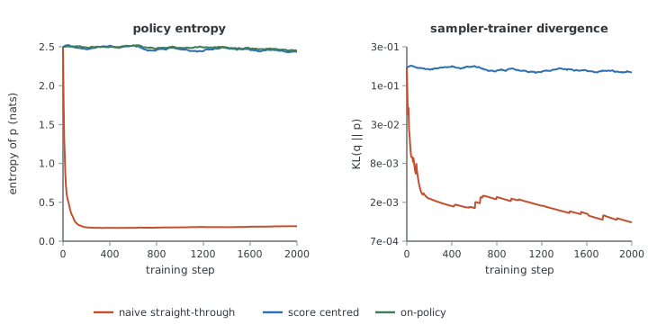
Policy entropy and sampler-trainer divergence under a constant reward. — Figure 1. Two thousand SGD steps under a constant reward with an int4 sampler, \(32{,}768\) token samples per step. There is no learning signal in this problem. The on-policy and score-centered runs random-walk and stay put; the naive straight-through run collapses the policy onto a single token. The naive run's divergence falls because it bought agreement with the sampler by destroying the policy — a near-deterministic distribution is one that quantization can no longer perturb. On-policy divergence is identically zero and cannot be drawn on a log axis.

estimator	entropy of \(p\)	top-1 probability	\(D_{\mathrm{KL}}(q \Vert p)\)
naive straight-through	\(2.500 \to 0.194\)	\(0.352 \to 0.977\)	\(1.7\times 10^{-1} \to 1.3 \times 10^{-3}\)
score centered	\(2.500 \to 2.438\)	\(0.352 \to 0.384\)	\(1.7\times 10^{-1} \to 1.5 \times 10^{-1}\)
on-policy	\(2.500 \to 2.451\)	\(0.352 \to 0.369\)	\(0 \to 0\)

Table 2. Start and end of the runs above. All three use the same learning rate, so the collapse is not a step-size artefact — the two controls are flat under identical settings.

The naive run has no reward signal to follow and follows something anyway, losing \(92\%\) of its entropy in about two hundred steps. Note what this experiment is: \(R \equiv 1\) and \(R \equiv 0\) differ by an additive constant, and on-policy they are the same problem. The naive estimator tells them apart. Reward-level invariance is not a nicety — it is the property whose failure produces this plot, and it is why the paper finds \(+1/0\) rewards the least stable online setting, the exact reverse of their offline ordering.

Drift is not instability you can tune away

The usual response to an RL run that degrades is to lower the learning rate, raise the batch size, or clip harder. None of those touch a bias. Lowering the learning rate slows the drift and the signal by the same factor. Raising the batch size, as the next section shows, makes the drift relatively worse.

The bias grows with compute

Per step, the drift contributes a fixed vector \(d\), independent of how many samples you drew. The noise contributes a zero-mean vector of norm \(\sigma/\sqrt{B}\) for \(B\) token samples. Accumulate \(T\) steps and the two behave differently — the drift adds coherently, the noise random-walks:

\[\frac{\lVert \text{accumulated drift} \rVert}{\lVert \text{accumulated noise} \rVert} = \frac{T \lVert d \rVert}{\sigma \sqrt{T / B}} = \sqrt{T B} \; \frac{\lVert d \rVert}{\sigma} .\]

\(TB\) is the total number of token samples the run has drawn. The bias-to-noise ratio of everything the run has done grows as the square root of total sample count, and it does not care how you split that count between steps and batch. Longer runs, bigger batches, more rollouts per prompt — every axis you scale up moves you further into the drift-dominated regime, and none of them average the drift away. Crossover comes at \(N^\star = (\sigma / \lVert d \rVert)^2\) samples.

batch \(B\)	total samples (\(T = 64\))	\(\lVert \sum_t \hat g_t \rVert\)	\(T \lVert d \rVert\)	drift's share
\(64\)	\(4{,}096\)	\(0.894\)	\(0.593\)	\(0.66\)
\(256\)	\(16{,}384\)	\(0.668\)	\(0.593\)	\(0.89\)
\(1{,}024\)	\(65{,}536\)	\(0.635\)	\(0.593\)	\(0.93\)
\(4{,}096\)	\(262{,}144\)	\(0.603\)	\(0.593\)	\(0.98\)
\(16{,}384\)	\(1{,}048{,}576\)	\(0.590\)	\(0.593\)	\(1.01\)

Table 3. Accumulated update over a fixed \(T = 64\) steps with an int8 sampler, under a constant reward so that the signal is exactly zero and the entire mean is drift. Mean of 8 seeds. Here \(\sigma / \lVert d \rVert = 97\), so \(N^\star \approx 9{,}500\) samples — the point at which accumulated bias and accumulated noise are equal. Past it the update is increasingly just the bias.

This is the quantitative form of an obstacle the paper hit experimentally. They report struggling to find natural setups with mismatch severe enough to separate the best methods in a few GPU hours, and deliberately amplify the mismatch as a proxy for long training under mild mismatch — because under mild mismatch it simply takes more steps for drift to accumulate. The \(\sqrt{N}\) law says that proxy is sound, and says what it trades: mismatch severity and total sample count enter the bias-to-noise ratio as a product, so you can buy severity with steps at a fixed exchange rate.

The toy understates the noise

This policy has a single context, so its gradient noise is far smaller than a real run's, where thousands of prompts and positions pull in different directions while the drift stays coherent. That pushes \(N^\star\) up, perhaps by orders of magnitude. The \(\sqrt{N}\) growth is algebra and does not move.

The repair

Score centering subtracts the mean, \(\hat g_{\text{sc}} = A(s_y - \mu)\). In the implementation this is a term \(\sum_v q(v) \log p_\theta(v)\) added to the per-token objective with \(q\) detached — the negative cross-entropy of the trainer against the sampler, which differentiates to exactly \(\mu\).

In logit space the result is startling. The naive estimator is \(A(e_y - p)\) and the correction is \(q - p\), so

\[\hat g_{\text{sc}} = A\left[(e_y - p) - (q - p)\right] = A\left(e_y - q\right).\]

The centered estimator is the exact score of the sampler, evaluated on the trainer's logits. The straight-through substitution replaced \(\nabla \log q\) by \(\nabla \log p\); centering puts \(q\) back at the softmax. Every consequence of the score identity returns with it: the expectation is a covariance, so a constant reward gives exactly zero, and shifting every advantage by \(c\) changes the expected gradient by \(c\,\mathbb{E}_q[e_y - q] = 0\).

The paper is careful to place this against the classical literature, and the distinction is worth repeating. Baselines (Williams, 1992) and score-function control variates both lean on \(\mathbb{E}_p[s] = 0\), but they are variance reductions that leave the mean alone. Score centering is a bias correction that shifts the mean, and the reason no one had written it down is that on-policy it is identically zero, while in classical off-policy RL the expected score is an intractable sum over the action space. LLM RL is the unusual case where it is both nonzero and exactly computable, because the action space is the vocabulary and the policy is a softmax over it.

Which gradient did you want?

Here is where the straight-through lens earns its keep, and it starts from the paper's own limitation. Score centering makes the expected update \(\mathrm{Cov}_q(A, s)\), whereas the on-policy update is \(\mathrm{Cov}_p(A, s)\). The covariance is measured under the sampler, not the trainer. The paper lists this as a residual defect and attributes to it their finding that under severe staleness, score centering composed with TIS or MIS beats score centering alone.

But whether that is a defect depends on a question nobody in this setup states out loud: which expectation were you trying to maximise?

If the target is \(\mathbb{E}_{p_\theta}[R]\) — the bf16 trainer's own return — then \(q\) is a nuisance, its only role is to have produced the samples, and \(\mathrm{Cov}_q\) instead of \(\mathrm{Cov}_p\) is exactly the leftover error the paper names.
If the target is \(\mathbb{E}_{q}[R]\) — what the quantized engine you actually serve will earn — then the whole setup is QAT, the correct gradient needs \(\nabla \log q\), and \(\mathrm{Cov}_q\) is the right measure. On this reading score centering is not an off-policy correction at all. It is the straight-through estimator with the substitution pushed out of the softmax and down into the logit Jacobian, where \(\partial \ell_q / \partial \theta\) is still being approximated by \(\partial \ell_p / \partial \theta\) — the same, much milder approximation that supervised QAT has always trained through.

The two readings make different predictions, and the split falls along the paper's two sources of mismatch. Under quantization, \(q\) is a model you plausibly deploy, so \(\mathrm{Cov}_q\) is defensible as a target and correcting it back toward \(p\) should buy little. Under staleness, \(q\) is a checkpoint from 64 steps ago that nobody will ever serve, so \(\mathrm{Cov}_q\) is simply the wrong measure and you should want importance sampling to drag it toward \(p\).

That is what their experiments show. Under quantization, score centering alone is competitive with its compositions; under staleness, the compositions clearly win. The paper reaches the staleness half of this from Equation 5. The QAT reading gets both halves, and says the asymmetry is not an accident of which mismatch is more severe but a statement about which distribution you were entitled to call the target. I have not tested this, and it is a conjecture consistent with their data rather than a result — the obvious experiment is to evaluate the quantized sampler rather than the trainer and see whether the ranking moves.

Importance sampling is the other repair, and you know the bill

There is a second way to restore the identity: fix the forward measure rather than the backward map, by reweighting each sample by \(r = p/q\). Then

\[\mathbb{E}_{y \sim q}\!\left[\frac{p(y)}{q(y)} \nabla_\theta \log p_\theta(y)\right] = \mathbb{E}_{y \sim p}\!\left[\nabla_\theta \log p_\theta(y)\right] = 0 ,\]

so exact importance sampling is drift-free, and the score centering correction under exact weights is identically zero — there is nothing left to cancel.

The trouble is that nobody runs exact importance sampling, and the previous post is the reason why: the variance of the weights is a \(\chi^2\) divergence, it compounds over tokens, and an untruncated sequence-level ratio is unusable at any realistic length. So every method in practice truncates — TIS clamps the ratio at \(2\), MIS keeps it on \([0.5, 5]\) and zeroes it outside, PPO clips to \([0.8, 1.2]\), DAPO to \([0.8, 1.28]\).

And truncation puts the bias straight back. The paper's Appendix A.2 gives the general correction: for weight function \(w\), centre against the expectation of the weighted score, \(\mathbb{E}_q[w_{y_t} s_{y_t}] = \sum_v q_v w_v s_v\). In the softmax picture that expectation is a vector you can name — the effective mass \(m(v) = q(v)\,w(p(v)/q(v))\) — and the drift is \(\bar A (m - \lVert m \rVert_1 p)\), which vanishes if and only if \(m \propto p\). Exact weights give \(m = q \cdot (p/q) = p\); any clipping or masking bends \(m\) away from \(p\).

estimator (int4 sampler)	\(\lVert \text{drift} \rVert\)	as % of signal	noise vs naive	\(q\)-mass reweighted
naive (plain STE)	\(2.10 \times 10^{-2}\)	\(27.7\%\)	\(1.00\times\)	\(1.000\)
naive + score centering	\(0\)	\(0.0\%\)	\(1.21\times\)	\(1.000\)
exact IS, \(w = r\)	\(0\)	\(0.0\%\)	\(2.84\times\)	\(0.000\)
TIS, clip at \(2\)	\(5.26 \times 10^{-3}\)	\(7.0\%\)	\(1.81\times\)	\(0.083\)
TIS + score centering	\(0\)	\(0.0\%\)	\(1.88\times\)	\(0.083\)
MIS, keep \(r \in [0.5, 5]\)	\(3.89 \times 10^{-4}\)	\(0.5\%\)	\(2.84\times\)	\(0.024\)
MIS + score centering	\(0\)	\(0.0\%\)	\(2.84\times\)	\(0.024\)
PPO, clip to \([0.8, 1.2]\)	\(1.40 \times 10^{-2}\)	\(18.5\%\)	\(1.14\times\)	\(0.912\)
PPO + score centering	\(0\)	\(0.0\%\)	\(1.29\times\)	\(0.912\)

Table 4. Exact drift and per-sample noise for each weighting, on the same policy. The drift a scheme leaves behind tracks how much of the sampler's mass its band touches. Score centering's correction is deterministic given the prefix, so it removes all the drift for a fifth more noise; importance sampling's is a random multiplicative factor, and removes the same drift for nearly triple.

Two things in that table are worth drawing out.

PPO's clip is the worst of both worlds under quantization. Its narrow band touches \(91\%\) of the sampler's mass, so it keeps two thirds of the drift while barely reducing variance. The paper observes that PPO and DAPO survive staleness but collapse under quantization and weight noise, and reads it as their clip being designed for ratios that come from policy movement rather than numerical error. The effective-mass picture says the same thing quantitatively: a band calibrated to policy movement is far too tight for the ratio spread that quantization produces, so it binds almost everywhere and behaves like no correction at all.

At mild mismatch the methods cannot separate. Run the same table at int8 and no ratio leaves \([0.8, 1.2]\) — every band is slack, every scheme collapses to exact importance sampling, and all of them have zero drift, centered or not. Methods can only separate once clipping actually binds, which is exactly where truncation starts trading bias for the variance it was brought in to control. That is the mechanism behind the paper's headline framing that the gap grows with the severity of the mismatch.

The identity that broke is the identity that pays for the fix

The correction \(\mu = q - p\) needs the sampler's distribution over the whole vocabulary, which is not a thing you can store. The paper does the arithmetic: Qwen3's vocabulary is 152K, so full fp32 logprobs for a batch of 1024 rollouts at 32K tokens would be 20TB. So they log the top \(k\) (\(k = 128\)) and model the tail with the trainer's distribution rescaled to match the sampler's tail mass, \(\hat q_v = \rho\, p_v\) on the tail.

Watch what that assumption buys. The tail's contribution to the correction is

\[\rho \sum_{v \in \text{tail}} p_v\, s_v = \rho\left[\underbrace{\textstyle\sum_{v \in \mathcal{V}} p_v s_v}_{=\;0} - \sum_{v \in \text{head}} p_v\, s_v\right],\]

so the whole tail collapses into a gather over the \(k\) head tokens and the backward pass never touches the full vocabulary. The identity that the straight-through substitution destroyed under \(q\) still holds under \(p\), and it is what pays for the repair — at \(k=128\), within \(1\%\) of the wall-clock time of the baseline methods.

It also explains why the tail must be modelled rather than dropped. Dropping it leaves \(\sum_v \hat q_v = m < 1\), and the correction becomes \(q_{\text{head}} - m\,p\) instead of \(q - p\); the leftover \((1-m)\,p\) is a drift term in its own right.

\(k\)	head mass under \(q\)	relative error, modelled tail	relative error, dropped tail
\(16\)	\(0.9148\)	\(0.072\)	\(0.284\)
\(32\)	\(0.9532\)	\(0.033\)	\(0.165\)
\(128\)	\(0.9903\)	\(0.007\)	\(0.036\)
\(512\)	\(0.9992\)	\(0.001\)	\(0.003\)
\(4096\) (full)	\(1\)	\(0\)	\(0\)

Table 5. Error in the correction relative to \(\lVert q - p \rVert_1\), int4 sampler. Modelling the tail is worth about a factor of five over dropping it at every \(k\); at \(k = 128\) the correction is \(99.3\%\) exact, consistent with the paper finding \(k = 128\) and even \(k = 32\) on par with full score centering.

Takeaways

RL under training–inference mismatch is quantization-aware training: forward through quantized weights, backward as though they were not. The estimator in use is a straight-through estimator, and the paper's drift is its bias.
For a softmax policy that bias is exactly \(q - p\), scaled by the expected advantage at the prefix. Per-prefix, not per-batch — which is why GRPO's group centering shrinks drift without removing it.
The identity that breaks is \(\mathbb{E}_p[\nabla \log p] = 0\), and with it goes invariance to the additive level of the reward. A constant reward will train the model, and in this toy it destroys \(92\%\) of the policy's entropy in two hundred steps.
Because it is a bias, batch size does not help. The bias-to-noise ratio of the accumulated update grows as \(\sqrt{N}\) in total samples drawn, however you split them — which is why amplifying mismatch is a sound proxy for training longer.
Score centering gives \(A(e_y - q)\): the sampler's exact score on the trainer's logits. Whether the residual \(\mathrm{Cov}_q\) is a defect or the target depends on whether you intend to serve the quantized model — and that, I suspect, is why quantization and staleness behave differently in their experiments.
Truncated importance sampling is a straight-through estimator whose de-biasing you undid on exactly the tokens where the mismatch was largest. That is why the two compose.

References

Marek and Ryabinin, 2026, "Score Centering Stabilizes Off-policy Reinforcement Learning" (code)
Bengio, Léonard, and Courville, 2013, "Estimating or Propagating Gradients Through Stochastic Neurons for Conditional Computation"
Courbariaux, Bengio, and David, 2015, "BinaryConnect: Training Deep Neural Networks with binary weights during propagations"
van den Oord, Vinyals, and Kavukcuoglu, 2017, "Neural Discrete Representation Learning"
Williams, 1992, "Simple statistical gradient-following algorithms for connectionist reinforcement learning"
Schulman, Wolski, Dhariwal, Radford, and Klimov, 2017, "Proximal Policy Optimization Algorithms"
Shao et al., 2024, "DeepSeekMath: Pushing the Limits of Mathematical Reasoning in Open Language Models"