The Variance of Importance Sampling
Post-training a language model involves an awkward fact: the samples you have were usually not drawn from the distribution you care about. The rollouts came from a policy that is a few gradient steps stale, or from a replay buffer, or from an inference engine whose numerics do not exactly match the trainer's. Call the distribution that actually produced the tokens \(q\), and the policy you want to reason about \(p\).
Importance sampling is the textbook repair, and it has one very attractive property: it is unbiased. But unbiasedness is the cheapest property in statistics. An estimator can be unbiased and still be wrong by a factor of three every single time you run it — and, worse, report a tight confidence interval while doing so.
This post works through two discrete examples small enough to compute by hand, and deliberately shaped like a language model, to show how fast this goes wrong. All numbers below come from simulations you can re-run in a few lines of Python.
The estimator
We want the mean of some \(f\) under \(p\),
but we can only draw \(x_1, \dots, x_N \sim q\). Importance sampling reweights each sample by the likelihood ratio \(w(x) = p(x)/q(x)\):
It is unbiased for any \(q\) that covers \(p\), by a one-line calculation:
Nothing in that line mentions how close \(q\) is to \(p\). The closeness shows up entirely in the second moment, which is where all of the trouble lives.
Failure 1: one rare token
Take the smallest vocabulary that can go wrong, \(\mathcal{V} = \{a, b\}\), and a reward that fires on one of them: \(f(a) = 1\), \(f(b) = 0\). The target policy is a coin flip, \(p(a) = p(b) = 0.5\), so the quantity we want is
Now suppose the policy we actually sampled from has drifted so that it almost never emits \(a\): \(q(a) = \delta = 10^{-3}\). The single interesting weight is
The estimator is honest — it is still unbiased — but look at its spread:
The standard deviation of a single sample is \(15.8\), about 32 times the quantity being estimated. With \(N = 100\) samples the standard error is still \(1.58\), or \(3.2\times\) the answer. I ran \(200{,}000\) independent replications of that \(N = 100\) estimate:
| statistic | value |
|---|---|
| mean of the estimates | \(0.5042\) (unbiased, as promised) |
| standard deviation | \(1.589\) |
| fraction that came out exactly \(0\) | \(90.4\%\) |
| median | \(0\) |
| 99th percentile | \(5.0\) |
| maximum observed | \(15.0\) |
This is the failure mode worth internalising. Nine times out of ten, the run never draws a single \(a\), the estimate is exactly \(0.000\), and the sample variance is also exactly zero. The estimator does not return "\(0\), but I am unsure." It returns "\(0 \pm 0\)" with total confidence, and it is wrong by the entire magnitude of the answer. The remaining \(10\%\) of runs hold all of the correctness, and they overshoot wildly — the occasional run reports \(15.0\) for a quantity that cannot exceed \(1\).
The tell is absent, not present
A high-variance importance sampling estimate does not usually announce itself with noisy numbers. It announces itself by being suspiciously quiet: the heavy tail that carries the truth is exactly the part you did not sample, so both your point estimate and your error bar are computed from the boring \(90\%\).
Why: the variance is a divergence
The reason is not specific to that example. Rewrite the second moment as an expectation under \(p\):
The weight \(w\) appears inside an expectation under \(p\). Specialise to \(f \equiv 1\) and you get a quantity that depends only on the mismatch between the two distributions:
So the variance of the weights is the \(\chi^2\) divergence between target and proposal. This gives the standard diagnostic, the effective sample size:
\(N\) samples from \(q\) are worth roughly \(N / (1 + \chi^2)\) samples from \(p\). In the example above \(1 + \chi^2 = 0.25/10^{-3} + 0.25/0.999 = 250.25\), so a batch of \(100{,}000\) mismatched rollouts buys you about \(400\) honest ones.
There is a sharper statement. Chatterjee and Diaconis (2018) show that the sample size needed for importance sampling to work is of order
and that below this threshold the estimate is typically off — not merely noisy, but concentrated on the wrong value. The cost is exponential in a divergence. Hold onto that, because in a language model the divergence is a sum over tokens.
Failure 2: a thousand tokens, each almost right
The first example needed a dramatic mismatch: a factor of \(500\) on a single token. Real policies are rarely that far apart. The sequence case does not need them to be.
Let both policies be i.i.d. over \(T\) steps on the same two-token vocabulary, with
A five-percentage-point difference on one token. No one would call these different policies. But the sequence weight is a product:
Both divergences are additive over the \(T\) steps, and for this symmetric pair they have closed forms:
Per token, \(D_{\mathrm{KL}} = 0.005\) nats — about seven thousandths of a bit, utterly negligible. Multiply by \(T\) and watch what that negligible quantity does. I drew \(N = 100{,}000\) sequences from \(q\) at each length:
| \(T\) | \(D_{\mathrm{KL}}(p \Vert q)\) | \(1 + \chi^2\) | measured ESS | median \(w\) | largest weight's share |
|---|---|---|---|---|---|
| \(1\) | \(0.005\) | \(1.01\) | \(99{,}000\) | \(0.91\) | \(0.0\%\) |
| \(10\) | \(0.050\) | \(1.11\) | \(90{,}464\) | \(0.86\) | \(0.0\%\) |
| \(100\) | \(0.503\) | \(2.73\) | \(36{,}096\) | \(0.61\) | \(0.1\%\) |
| \(1000\) | \(5.025\) | \(23{,}160\) | \(12.2\) | \(0.0067\) | \(22.5\%\) |
Table 1. Importance sampling between two policies that differ by \(0.05\) in probability on every token. At \(T = 1000\) the \(100{,}000\) sampled sequences are worth about a dozen, and a single sequence carries nearly a quarter of the total weight.
At \(T = 1000\) the estimator has collapsed. \(1 + \chi^2 \approx 23{,}000\) means you need roughly \(23{,}000\) rollouts to buy one effective sample. One sequence out of \(100{,}000\) holds \(22.5\%\) of the weight — the "average" is being computed from a handful of points.
The mechanism is visible in the shape of \(\log w\). Here it is a sum of \(T\) i.i.d. terms, so the CLT applies and \(w\) is approximately log-normal: \(\log w \sim \mathcal{N}(-5.01,\, 3.16^2)\). The approximation is essentially exact — it predicts a median weight of \(0.006682\), and the simulated median is \(0.006682\). For a log-normal the mean sits a full \(\sigma^2\) above the median in log space, and \(\sigma^2\) grows linearly in \(T\):
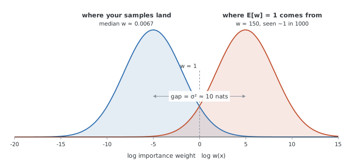
Figure 1. The distribution of \(\log w\) at \(T = 1000\) (blue) against the distribution of where the mass of \(\mathbb{E}[w] = 1\) actually comes from (red). The two are separated by \(\sigma^2 \approx 10\) nats, roughly three standard deviations.
Real policies are autoregressive, so their per-token log-ratios are neither independent nor identically distributed and the log-normal shape is a convenience of this example. The part that matters survives the generalisation: \(\log w\) is a sum over tokens, so both its drift and its spread accumulate with length, and \(w\) stays skewed enough that the mean and the typical value part company.
Every sampled sequence is, individually, entirely typical. And \(94\%\) of them have \(w < 1\). The estimator is unbiased only because of sequences at \(w \approx 150\) that show up about once in a thousand draws, and sequences at \(w \approx 40{,}000\) that show up essentially never. Concretely, out of \(200{,}000\) samples:
| slice of samples | share of total weight |
|---|---|
| top \(0.01\%\) (20 sequences) | \(39.8\%\) |
| top \(0.1\%\) | \(61.9\%\) |
| top \(1\%\) | \(83.4\%\) |
| top \(10\%\) | \(97.5\%\) |
Watching it wreck a real estimate
Divergences and ESS are abstract, so here is the damage on an actual quantity. Keep the same \(p\), \(q\), and \(T = 1000\), and let
Under \(p\) this is a coin-flip question and the true value is \(\mathbb{E}_p[f] = 0.4874\), computable exactly. Under \(q\) it is a tail event with probability \(0.00068\). Eight independent runs, each with \(N = 100{,}000\) sequences:
| run | ESS | importance sampling estimate | self-normalised estimate |
|---|---|---|---|
| 1 | \(12.0\) | \(0.858\) | \(0.624\) |
| 2 | \(65.3\) | \(0.480\) | \(0.480\) |
| 3 | \(172.8\) | \(0.438\) | \(0.455\) |
| 4 | \(37.9\) | \(0.673\) | \(0.570\) |
| 5 | \(8.2\) | \(\mathbf{1.294}\) | \(0.721\) |
| 6 | \(231.0\) | \(0.316\) | \(0.375\) |
| 7 | \(131.2\) | \(0.380\) | \(0.425\) |
| 8 | \(28.6\) | \(0.501\) | \(0.483\) |
Table 2. Estimating a quantity whose true value is \(0.4874\), using \(100{,}000\) importance-weighted samples per run.
A hundred thousand samples, and the estimates range from \(0.32\) to \(1.29\) — a factor of four. Run 5 reports \(1.294\) for a probability, which is a useful kind of failure because it is visibly impossible. Runs 3, 6 and 7 report \(0.44\), \(0.32\) and \(0.38\), which are wrong by \(10\)–\(35\%\) and look completely plausible. Those are the dangerous ones.
It is tempting to answer that unbiasedness will save you if you average. Average all eight runs — \(800{,}000\) samples — and you get \(0.617\), still \(27\%\) high. Unbiasedness is a statement about a limit, and when a few extreme weights carry most of the mass, that limit is a very long way off. In any case, you do not get to average eight training runs.
Your diagnostics are computed from the same bad samples
One more twist. The theoretical ESS at \(T = 1000\) is \(N / (1 + \chi^2) \approx 4\). The measured ESS in the table above ranges from \(8\) to \(231\) — consistently optimistic, by up to two orders of magnitude.
This is not a bug in the estimator; it is the same problem one level up. \(\widehat{\mathrm{ESS}}\) depends on \(\sum_i w_i^2\), which is dominated by the extreme tail of \(w\) — the part you almost certainly did not sample. A run that misses the tail reports a comfortable ESS because it missed the tail. The diagnostic degrades precisely when you need it, and in the reassuring direction.
The practical consequence: treat a measured ESS as an upper bound. If it already looks bad, things are worse than it says.
What actually helps
Keep \(q\) close to \(p\). This is the only fix that addresses the cause rather than the symptom, because the cost is exponential in a divergence that accumulates per token. In the example, halving \(\epsilon\) to \(0.025\) divides the per-token KL by four and takes \(1 + \chi^2\) at \(T = 1000\) from \(23{,}000\) down to \(12\). Everything that shrinks the mismatch — refreshing rollouts more often, KL penalties or trust regions, making the inference engine and the trainer agree numerically — buys back sample efficiency at an exponential rate. This is why a "small" discrepancy between a sampling stack and a training stack is not small: it is a per-token quantity multiplied by the sequence length.
Don't form the length-\(T\) product. The product over tokens is what turns a negligible per-step divergence into an exponential one. Policy-gradient objectives in the PPO family (Schulman et al., 2017) and their LLM descendants such as GRPO (Shao et al., 2024) apply a per-token ratio \(\pi_\theta(x_t \mid x_{<t}) / \pi_{\text{old}}(x_t \mid x_{<t})\) against a per-token advantage, rather than one sequence-level weight. This is no longer an unbiased importance sampling estimate of the sequence-level objective; it trades a bias you can reason about for a variance that does not compound with length.
Clip, but know what you are buying. Replacing \(w\) with \(\min(w, c)\) bounds the variance by construction, and the bias it introduces can be every bit as bad as the variance it removes. In Failure 1, where the true value is \(0.5\) and \(w(a) = 500\):
| clip \(c\) | \(\mathbb{E}[\text{clipped estimator}]\) | bias |
|---|---|---|
| \(1\) | \(0.0010\) | \(-0.499\) |
| \(10\) | \(0.0100\) | \(-0.490\) |
| \(100\) | \(0.1000\) | \(-0.400\) |
| \(500\) | \(0.5000\) | \(0\) |
Clipping at \(c = 10\) turns a wild but correct-on-average estimator into a calm one that reports \(0.01\) for a quantity equal to \(0.5\). Clipping is safe when the weights were mostly fine and you are trimming a few outliers; it is a disguise when they were not. Truncating at a level that grows with \(N\) (Ionides, 2008) makes the bias vanish asymptotically, and Pareto-smoothed importance sampling (Vehtari et al., 2015) fits a generalised Pareto to the tail instead of truncating it — its fitted shape parameter \(\hat{k}\) is a far better diagnostic than ESS, with \(\hat{k} > 0.7\) meaning the estimate should not be trusted.
Self-normalise. Dividing by \(\sum_i w_i\) instead of \(N\) introduces an \(O(1/N)\) bias but confines the estimate to the range of \(f\). In the table above it pulls run 5 from the impossible \(1.294\) back to \(0.721\) and tightens the overall spread from \([0.32, 1.29]\) to \([0.38, 0.72]\). Still bad — it cannot manufacture information that is not in the samples — but no longer nonsensical.
Takeaways
- Importance sampling is unbiased for any proposal that covers the target. Unbiasedness says nothing about whether a given run is close to the answer.
- The variance of the weights is a divergence: \(\mathrm{Var}_q[w] = \chi^2(p \,\Vert\, q)\), and the sample size you need scales like \(e^{D_{\mathrm{KL}}(p \Vert q)}\).
- For sequences, the weight is a product over tokens, so the divergence is a sum over tokens and the cost is exponential in the sequence length. A \(0.05\) per-token gap is fatal at \(T = 1000\).
- The characteristic failure is silent: the tail that carries the truth is the part you did not sample, so the point estimate and the error bar and the ESS are all computed from the well-behaved majority and all agree with each other.
- Treat measured ESS as an optimistic upper bound. Prefer \(\hat{k}\) from PSIS if you can.
References
- Chatterjee and Diaconis, 2018, "The sample size required in importance sampling"
- Owen, 2013, "Monte Carlo theory, methods and examples", Chapter 9
- Ionides, 2008, "Truncated importance sampling"
- Vehtari, Simpson, Gelman, Yao, and Gabry, 2015, "Pareto smoothed importance sampling"
- Schulman, Wolski, Dhariwal, Radford, and Klimov, 2017, "Proximal Policy Optimization Algorithms"
- Shao et al., 2024, "DeepSeekMath: Pushing the Limits of Mathematical Reasoning in Open Language Models"