Policy Gradients and the Arithmetic of Variance
The policy gradient theorem is about four lines of algebra, and almost none of the work in making it function is in those four lines. The derivation gives you an estimator that is unbiased for any policy, any reward, any dynamics — including dynamics you cannot differentiate and rewards you cannot write down. Then you run it and nothing happens, because the estimator's variance is large enough to bury the signal it is carrying.
This post derives the gradient in Pieter Abbeel's notation, then treats variance as the actual subject. The claim I want to make precise is the one usually waved at: subtracting a baseline reduces variance. That is a theorem with an explicit form, an exactly optimal \(b^\star\), and a characterisation of which baselines help and which hurt — and the standard choice, the mean return, is not the optimal one.
Every number below comes from a simulation or an exact enumeration, and the closed forms are checked against Monte Carlo before they are stated.
Setup and notation
A trajectory is the whole rollout — states and controls, from reset to horizon:
Following Abbeel's lectures I write \(u_t\) for the action, a habit inherited from optimal control; if you learned this as \(a_t\), they are the same object. The policy \(\pi_\theta(u \mid s)\) is stochastic and parameterised by \(\theta\), and we want to maximise the expected return of a rollout,
where \(R(\tau) = \sum_{t=0}^H R(s_t,u_t)\) is the return of a single trajectory and \(P(\tau;\theta)\) is the probability that rolling out \(\pi_\theta\) produces \(\tau\). The sum over \(\tau\) is notation, not an algorithm — the space of trajectories is astronomical, and the entire point of what follows is to estimate this from \(m\) sampled rollouts.
The derivation
We want \(\nabla_\theta U(\theta)\). The obstacle is that \(\theta\) sits inside the distribution we are averaging over, not inside the thing being averaged. Push the gradient through the sum and multiply by \(1 = P(\tau;\theta)/P(\tau;\theta)\):
The ratio is the gradient of a logarithm, \(\nabla_\theta \log P(\tau;\theta)\), which turns the sum back into an expectation over trajectories:
An expectation is something we can sample. With \(m\) rollouts \(\tau^{(1)},\dots,\tau^{(m)}\) drawn from the current policy:
This is the likelihood ratio estimator, and it is unbiased by construction: \(\mathbb{E}[\hat g] = \nabla_\theta U(\theta)\) exactly, for any \(m \geq 1\).
The dynamics cancel
\(\log P(\tau;\theta)\) still looks like it needs a model of the world. It does not. Write out the trajectory probability as the product of dynamics and policy,
take logs to turn the product into a sum, and differentiate:
The dynamics terms have no \(\theta\) in them, so they differentiate to zero. What remains is a quantity you can compute from the policy network alone. Substituting back:
Three things this bought us, all of which follow from \(R(\tau)\) appearing only as a multiplicative scalar. The estimator needs no model of the environment. It never differentiates \(R\), so the reward may be discontinuous, discrete, or a black box — a human preference, a unit test passing, a simulator crashing. And it never differentiates the dynamics either, so the environment can be equally unfriendly.
What it is actually doing
Read the estimator as a weighted maximum likelihood update. The term \(\nabla_\theta \log \pi_\theta(u_t \mid s_t)\) points in the direction that makes the action we took more likely; \(R(\tau)\) scales it. Good trajectories get their actions reinforced, bad ones get theirs suppressed.
Two consequences are worth holding onto, because they are the seeds of everything below. First, the weight is \(R(\tau)\), the return of the whole trajectory, applied to every action in it — including the actions taken after the rewards were collected. Second, the estimator is sensitive to the absolute level of \(R\), not just its variation across trajectories. Adding \(100\) to every reward leaves the optimal policy untouched and leaves \(\nabla_\theta U\) untouched, but it does not leave \(\hat g\) untouched at all.
Why variance is the whole story
Before fixing anything, it is worth being concrete about what a high-variance gradient costs, because "it converges more slowly" undersells it.
The smallest possible example
Take a one-step problem with a scalar Gaussian policy \(\pi_\theta(u) = \mathcal{N}(\theta, \sigma^2)\) and the linear reward \(R(u) = u + c\), where \(c\) is a constant. The score function is \(\nabla_\theta \log \pi_\theta(u) = (u - \theta)/\sigma^2\), and the true gradient is \(\nabla_\theta U = \nabla_\theta(\theta + c) = 1\), independent of \(c\).
Write \(u = \theta + \sigma \epsilon\) with \(\epsilon \sim \mathcal{N}(0,1)\). Then a single-sample estimate with baseline \(b\) is
and since \(\mathbb{E}[\epsilon] = \mathbb{E}[\epsilon^3] = 0\), \(\mathbb{E}[\epsilon^2] = 1\) and \(\mathrm{Var}[\epsilon^2] = 2\), the mean and variance are available in closed form:
At \(\theta = 0\), \(\sigma = 1\):
| \(c\) | \(b\) | \(\mathrm{Var}[\hat g]\) | \(\mathrm{sd}[\hat g]\,/\,\nabla_\theta U\) | rollouts for \(10\%\) relative error |
|---|---|---|---|---|
| \(0\) | \(0\) | \(2\) | \(1.41\) | \(200\) |
| \(100\) | \(0\) | \(10{,}002\) | \(100.0\) | \(1{,}000{,}200\) |
| \(100\) | \(100\) | \(2\) | \(1.41\) | \(200\) |
Table 1. A constant added to the reward does not change the problem, the optimum, or the gradient. It changes the number of rollouts needed to estimate that gradient by a factor of \(5{,}001\).
Nothing about the task changed between rows one and two. The optimal policy is the same, the true gradient is the same, and the second row costs five thousand times more experience. This is the entire argument for baselines in one table, and note that the third row recovers the original cost exactly by subtracting the mean return.
Variance is not a property of the problem
It is a property of the estimator you chose for a fixed problem. Two estimators of the same gradient, both perfectly unbiased, can differ by orders of magnitude in how much data they need. Reward scale, horizon, and policy entropy all move the variance around without moving the quantity being estimated.
Watching it break a training run
The table is a statement about one gradient evaluation. Here is the same effect inside an actual optimisation. Keep \(\pi_\theta = \mathcal{N}(\theta, 1)\), and use a reward with an interior optimum so there is something to converge to:
The optimum is \(\theta^\star = 3\) for every \(c\). Running REINFORCE with \(m = 16\) trajectories per update, a learning rate of \(0.02\), \(600\) updates, from \(\theta_0 = 0\), across \(200\) seeds:
| setting | final \(\theta\) (mean) | sd across seeds | median \(\lvert \theta - \theta^\star \rvert\) | within \(0.2\) of \(\theta^\star\) |
|---|---|---|---|---|
| \(c = 0\), no baseline | \(3.008\) | \(0.067\) | \(0.045\) | \(100\%\) |
| \(c = 100\), no baseline | \(2.732\) | \(1.702\) | \(1.207\) | \(10\%\) |
| \(c = 100\), batch-mean baseline | \(3.005\) | \(0.054\) | \(0.038\) | \(100\%\) |
Table 2. The same problem, three times. Adding \(100\) to a reward that the agent cannot influence takes a method that solves the task in every seed to one that solves it in one seed out of ten.
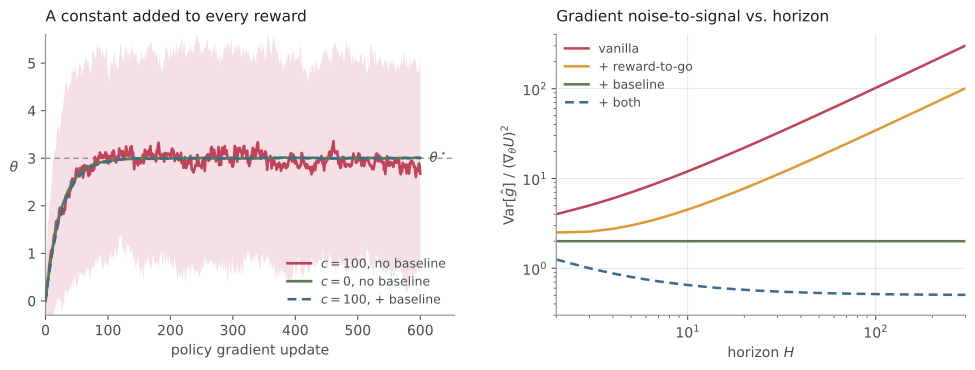
Figure 1.Left: median \(\theta\) over \(200\) seeds, with the \(10\)–\(90\%\) band shaded for the broken run. The median of the \(c = 100\) run looks converged; the individual runs are spread from \(\theta = 0.5\) to \(\theta = 5.0\) (10th to 90th percentile at the final update). Right: the closed-form noise-to-signal ratio \(\mathrm{Var}[\hat g] / (\nabla_\theta U)^2\) from the horizon analysis below, on log axes.
The left panel shows the characteristic shape. The median trajectory of the broken run is basically fine — it reaches \(\theta \approx 3\) and stays there. It is the spread that is catastrophic, and the spread is what you experience when you get one seed and one run.
Three mechanisms are doing the damage, and they are worth separating:
Individual updates point the wrong way. With \(c = 100\) at \(\theta = 0\), the true gradient is \(6.0\) and the standard deviation of a \(16\)-trajectory batch estimate is \(22.1\). About \(39\%\) of updates move away from the optimum. At the optimum the true gradient is \(0\) and the noise is still \(24.3\), so at the optimum the policy is driven entirely by a random walk whose steps are \(\pm 0.49\) in \(\theta\). It wanders away until the restoring gradient \(-2(\theta - 3)\) grows big enough to balance the noise, which happens at a spread of about \(1.7\) — the shaded band.
You cannot fix it by lowering the learning rate. The obvious response to a jittering parameter is a smaller step. It trades one failure for another:
| learning rate | final \(\theta\) (mean) | sd across seeds | median \(\lvert \theta - \theta^\star \rvert\) |
|---|---|---|---|
| \(0.02\) | \(2.938\) | \(1.777\) | \(1.240\) |
| \(0.005\) | \(2.974\) | \(0.858\) | \(0.576\) |
| \(0.001\) | \(2.105\) | \(0.358\) | \(0.908\) |
| \(0.0002\) | \(0.644\) | \(0.097\) | \(2.360\) |
Table 3.\(c = 100\), no baseline. Shrinking the step size buys precision and spends progress: at \(\alpha = 0.0002\) the policy is beautifully stable and has covered a fifth of the distance to the optimum in \(600\) updates.
Noise forces \(\alpha \sim 1/\mathrm{Var}\), and the number of updates to cover a fixed distance scales as \(1/\alpha\). Variance shows up as wall-clock time whether you accept the jitter or suppress it.
And in RL the damage compounds. This is the part with no supervised-learning analogue. A noisy gradient in supervised learning perturbs your parameters; the next minibatch is drawn from the same fixed dataset regardless. In RL the policy generates its own data, so a bad update changes the distribution of states you will visit next, which changes the gradient you estimate next. A policy knocked into a region it has no reason to be in will collect uninformative rollouts there, and for a Gaussian policy with a learned \(\sigma\) the usual outcome is worse: noise that shrinks \(\sigma\) prematurely reduces exploration, which raises the variance of everything downstream and welds the policy in place. Nothing in the objective is pulling it back out.
Fix 1: baselines, and the explicit variance
Define the trajectory score, which is the only \(\theta\)-dependent object in the estimator:
The baselined estimator subtracts a constant from the return before weighting:
It stays unbiased
The subtracted term vanishes in expectation, for any \(b\) not depending on \(\tau\):
Read it right to left: probabilities sum to one whatever \(\theta\) is, so the gradient of that sum is zero, so the expected score is zero. Everything in this post rests on that one line.
The explicit variance
Work coordinate by coordinate; let \(g_j\) denote the \(j\)-th component of \(g(\tau)\) and \((\nabla_\theta U)_j\) the corresponding true gradient. For a single sample,
The second term is fixed by unbiasedness, so choosing \(b\) means minimising the first. Expand it as a quadratic in \(b\):
Since \(\mathbb{E}[g_j^2] > 0\) this is a convex parabola, so setting \(\phi'(b) = 0\) gives the minimiser outright:
The optimal baseline is the return weighted by the squared magnitude of the score — not the plain average return. Trajectories whose actions the policy finds surprising get more say in setting the baseline, because those are the trajectories whose score is large and therefore whose contribution to the variance is large.
Completing the square in \(\phi\) gives the identity that does the real work:
Three statements fall out of it immediately.
The reduction at the optimum is explicit. Setting \(b = 0\) and \(b = b^\star_j\) and subtracting,
This is a ratio of a square to a positive number, so it is non-negative always, with equality only in the degenerate case \(\mathbb{E}[g_j^2 R] = 0\). That is the proof that an optimal baseline cannot hurt — and it quantifies exactly how much it helps.
Not every baseline helps. The identity says \(\mathrm{Var}(b) - \mathrm{Var}(0) = \mathbb{E}[g_j^2]\, b\,(b - 2b_j^\star)\), and since \(\mathbb{E}[g_j^2] > 0\) this is negative precisely when \(b\) lies strictly between \(0\) and \(2b_j^\star\):
Overshoot past twice the optimal baseline and you are increasing variance relative to using none at all. A baseline is not a free-form knob; it is a quantity with a right answer and a window around it, and the window is symmetric about \(b_j^\star\) only in the sense that the parabola is.
The optimum is per-coordinate. \(b^\star_j\) depends on \(j\), so a single scalar baseline cannot be optimal for every parameter at once. In practice everyone uses one scalar anyway, which is a small, deliberate concession.
The mean return is not the optimal baseline
It is standard to use \(b = \frac{1}{m}\sum_i R(\tau^{(i)})\), the batch mean. That is an estimate of \(\mathbb{E}[R]\), and \(\mathbb{E}[R] \neq b^\star\) in general. The gap can be most of the available reduction.
A two-armed bandit is enough to see it. Let \(\pi_\theta\) be a softmax over a single logit \(\theta\) with \(\pi(u_1) = p\), \(\pi(u_2) = 1 - p\). The scores are \(g(u_1) = 1-p\) and \(g(u_2) = -p\), so \(\mathbb{E}[g^2] = p(1-p)\) and
The optimal baseline weights the rewards by the opposite probabilities — again because what matters is the score magnitude, which is largest for the action the policy rarely takes. With \(p = 0.9\), \(r_1 = 0\), \(r_2 = 10\):
| baseline \(b\) | value | \(\mathrm{Var}[\hat g]\) | reduction achieved |
|---|---|---|---|
| none | \(0\) | \(7.29\) | — |
| mean return \(\mathbb{E}[R]\) | \(1.0\) | \(5.76\) | \(21\%\) |
| optimal \(b^\star\) | \(9.0\) | \(0\) | \(100\%\) |
Table 4. Two-armed bandit, \(p = 0.9\), rewards \((0, 10)\), true gradient \(-0.9\). The mean return is \(1.0\); the variance-optimal baseline is \(9.0\).
\(b^\star = 9\) drives the variance to exactly zero: the estimator returns \(-0.9\) on both arms, which is the true gradient, deterministically. That exactness is special to the two-outcome case — with two outcomes and one free parameter there is always a \(b\) that equates them — but the direction of the effect is not, and neither is the size of the gap. The conventional choice captured a fifth of what was on the table.
This is Weaver and Tao (2001) and Greensmith, Bartlett and Baxter (2004). The practical reason to keep using the mean anyway: estimating \(b^\star\) requires a second moment of the score per parameter, the estimate is itself noisy, and a noisy baseline correlated with the returns in your batch reintroduces bias. The mean return is robust, free, and usually gets you most of the way — usually, not always.
Fix 2: exploiting temporal structure
Return to the full estimator and look at what the trajectory return is multiplying:
The action at time \(t\) is being credited with rewards collected at times \(k < t\). It cannot have caused them. And by the same argument that killed the baseline term, those cross terms are zero in expectation — for \(k < t\), the reward \(r_k\) is a function of variables realised before \(u_t\) was sampled, so conditioning on everything up to time \(t\) and using \(\mathbb{E}[\nabla_\theta \log \pi_\theta(u_t \mid s_t) \mid s_t] = 0\) gives
They contribute nothing to the mean and plenty to the variance. Dropping them leaves each action weighted by its reward-to-go:
This is GPOMDP (Baxter and Bartlett, 2001), and it combines with a baseline that may now depend on time:
How much each fix is worth, as a function of horizon
Both fixes are usually justified by hand-waving. They can be computed. Take an \(H\)-step chain of identical bandits: at each step \(u_t \sim \mathcal{N}(\theta, \sigma^2)\) and \(r_t = u_t\), so \(U(\theta) = H\theta\) and \(\nabla_\theta U = H\). Writing \(u_t = \theta + \sigma\epsilon_t\) and using \(\mathbb{E}[\epsilon^2]=1\), \(\mathbb{E}[\epsilon^4]=3\), the four variants have exact variances:
The structure is legible. The vanilla estimator carries a term growing as \(H^3\); the optimal constant baseline here is \(b^\star = H\theta = \mathbb{E}[R]\) and it deletes that term outright, leaving \(O(H^2)\). Reward-to-go attacks the same term but only divides it by three, since \(\sum_{j=1}^H j^2 = H(H+1)(2H+1)/6 \approx H^3/3\). Relative to a gradient of size \(H\), the vanilla noise-to-signal ratio grows linearly in the horizon, while both baselined variants stay bounded — flat at \(2\) with a constant baseline, and decreasing to \(1/2\) with both fixes. That is the right panel of the figure above.
At \(H = 100\), \(\theta = 1\), \(\sigma = 1\), where the true gradient is \(100\):
| estimator | \(\mathrm{Var}[\hat g]\) | \(\mathrm{sd}\,/\,\lVert\nabla_\theta U\rVert\) | rollouts for \(10\%\) error | \(\Pr[\text{single rollout points the wrong way}]\) | reduction |
|---|---|---|---|---|---|
| vanilla | \(1{,}020{,}000\) | \(10.10\) | \(10{,}200\) | \(0.500\) | \(1\times\) |
| + reward-to-go | \(343{,}500\) | \(5.86\) | \(3{,}435\) | \(0.457\) | \(3.0\times\) |
| + baseline | \(20{,}000\) | \(1.41\) | \(200\) | \(0.000\) | \(51\times\) |
| + both | \(5{,}150\) | \(0.72\) | \(52\) | \(0.000\) | \(198\times\) |
Table 5. Closed forms, each confirmed against \(2 \times 10^6\) Monte Carlo rollouts to three significant figures. The sign probabilities are measured, not Gaussian approximations.
The wrong-way column is the one I find most useful. The vanilla estimator sends a single trajectory in the wrong direction half the time — it is, per rollout, indistinguishable from noise, and only averaging over thousands of rollouts extracts a direction. Add both fixes and the estimator provably never changes sign, because it reduces to \(\left(\sum_t \epsilon_t^2 + (\sum_t \epsilon_t)^2\right)/2 \geq 0\).
Note also which fix matters more. Reward-to-go alone buys \(3\times\); the baseline alone buys \(51\times\). Causality is the more intuitive correction and the less valuable one.
Fix 3: state-dependent baselines, and the actor-critic
Nothing forced \(b\) to be constant. The unbiasedness argument runs identically if \(b\) depends on the state, because the expected score conditioned on the state is still zero:
The natural choice is the value function \(b(s_t) = V^{\pi_\theta}(s_t) = \mathbb{E}[G_t \mid s_t]\), which makes the weight on each action the advantage:
Now the question each action is judged on is not "was the return large?" but "was this action better than what this policy usually does here?" — which is the question that actually carries information about \(\theta\). Fitting \(V\) with a second network is the actor-critic family (Sutton et al., 2000; Mnih et al., 2016).
To check all of this against something that is not a bandit, here is a \(2\)-state, \(2\)-action MDP with \(H = 4\) and a softmax policy, small enough that all \(256\) trajectories can be enumerated and every expectation computed exactly — no sampling:
| estimator | max \(\lvert\)bias\(\rvert\) | total variance | reduction |
|---|---|---|---|
| vanilla | \(0\) | \(17.43\) | \(1\times\) |
| + reward-to-go | \(<10^{-15}\) | \(7.54\) | \(2.3\times\) |
| + constant \(b = \mathbb{E}[R]\) | \(<10^{-15}\) | \(3.89\) | \(4.5\times\) |
| + state baseline \(V(s_t)\) | \(<10^{-15}\) | \(2.00\) | \(8.7\times\) |
| + action baseline \(Q(s_t,u_t)\) | \(\mathbf{0.615}\) | \(1.27\) | \(13.7\times\) |
Table 6. Exact expectations over all trajectories. The true gradient's largest component is \(0.615\). Biases at \(10^{-15}\) are floating-point zero.
The ordering confirms the bandit analysis, and the last row is a trap worth walking into deliberately. Making the baseline depend on the action as well as the state gives the lowest variance in the table — and a bias of \(0.615\), which is exactly the magnitude of the largest true gradient component. The estimator's mean is not merely wrong; it is identically zero, to machine precision, in every coordinate. Of course it is: \(\mathbb{E}[G_t \mid s_t, u_t] = Q(s_t,u_t)\), so subtracting \(Q\) centres the weight on every action, and there is no cheaper way to achieve zero variance than to estimate nothing at all.
Low variance is not the objective
The objective is low error. An estimator that returns \(0\) every time has zero variance and is useless. Action-dependent baselines need an explicit correction term to stay unbiased, and Tucker et al. (2018) found that several published methods in this family owed their reported gains to implementation details rather than to the action dependence — when the bias is correctly removed, most of the advantage goes with it.
Fix 4: discounting, and interpolating with GAE
The last standard knob is deliberately biased. Replacing the reward-to-go with its discounted version,
downweights rewards far in the future. The justification is that a reward \(50\) steps after an action is mostly not caused by it, so the \(\gamma^{k-t}\) factor strips noise whose expected contribution is small. This is no longer an unbiased estimator of \(\nabla_\theta U\), which is the point. On the same tabular MDP, using \(V\) as the baseline:
| \(\gamma\) | max \(\lvert\)bias\(\rvert\) | total variance |
|---|---|---|
| \(1.00\) | \(0\) | \(2.000\) |
| \(0.99\) | \(0.0013\) | \(1.963\) |
| \(0.95\) | \(0.0067\) | \(1.827\) |
| \(0.90\) | \(0.0135\) | \(1.681\) |
| \(0.70\) | \(0.0408\) | \(1.294\) |
| \(0.50\) | \(0.0685\) | \(1.114\) |
Table 7. A clean monotone trade. Against a largest gradient component of \(0.615\), \(\gamma = 0.99\) costs \(0.2\%\) bias for a \(2\%\) variance reduction; \(\gamma = 0.5\) costs \(11\%\) bias for \(44\%\).
The trade is smooth and it is a genuine trade — there is no setting of \(\gamma < 1\) that is free. Which end you want depends on how far your rewards actually are from the actions that caused them, which is a property of the environment and not something to inherit from a config file.
Generalised advantage estimation (Schulman et al., 2015) makes this an explicit dial. Write the TD residual \(\delta_t = r_t + \gamma V(s_{t+1}) - V(s_t)\) and take an exponentially weighted average of the \(n\)-step advantage estimators:
At \(\lambda = 1\) this telescopes back to \(G_t^\gamma - V(s_t)\): unbiased with respect to the discounted objective, high variance. At \(\lambda = 0\) it is the single residual \(\delta_t\): minimum variance, biased by whatever error \(V\) carries. Between them you are choosing how many steps of real reward to trust before handing off to the critic's guess — the same bias-variance trade as \(\gamma\), but decoupled from it, so the discount can stay a statement about the problem while \(\lambda\) stays a statement about your critic.
What to take from the arithmetic
The estimator falls out of a change of variables and is unbiased for anything. What makes it work is a sequence of modifications that leave the mean alone and attack the second moment: drop the terms that are zero in expectation, subtract what you could have predicted, and trade a controlled amount of bias for a large amount of variance where the causal link is weak anyway.
Takeaways
- The policy gradient is \(\nabla_\theta U(\theta) = \mathbb{E}_\tau[\nabla_\theta \log P(\tau;\theta) R(\tau)]\), and \(\nabla_\theta \log P(\tau;\theta) = \sum_t \nabla_\theta \log \pi_\theta(u_t \mid s_t)\) — the dynamics differentiate away, so no model is needed and \(R\) never has to be differentiable.
- Every variance reduction in this post rests on one identity: \(\mathbb{E}[\nabla_\theta \log P(\tau;\theta)] = 0\), because probabilities sum to one for every \(\theta\).
- The variance is an exact quadratic in the baseline: \(\mathrm{Var}(b) = \mathrm{Var}(b^\star) + \mathbb{E}[g_j^2](b - b_j^\star)^2\) with \(b_j^\star = \mathbb{E}[g_j^2 R]/\mathbb{E}[g_j^2]\). The reduction at the optimum is \((\mathbb{E}[g_j^2R])^2/\mathbb{E}[g_j^2] \geq 0\) — a baseline provably cannot hurt at \(b^\star\), and helps for any \(0 < b < 2b_j^\star\).
- \(b^\star\) weights returns by squared score magnitude, so it is not the mean return. In the worked bandit the mean return captured \(21\%\) of the available reduction and \(b^\star\) captured \(100\%\).
- A constant added to every reward changes no optimum and no gradient, and cost \(5{,}001\times\) more rollouts in the example — and broke \(90\%\) of training runs. Reward offsets are not cosmetic.
- Over a horizon, vanilla noise-to-signal grows linearly in \(H\). A baseline flattens it (\(51\times\) at \(H=100\)); reward-to-go alone only divides the leading term by three (\(3\times\)). The baseline is the bigger win.
- Low variance is not the goal. The \(Q\)-baseline achieves the lowest variance in the table by estimating exactly zero.
References
- Williams, 1992, "Simple statistical gradient-following algorithms for connectionist reinforcement learning"
- Abbeel and Schulman, "Deep Reinforcement Learning through Policy Optimization", NeurIPS 2016 tutorial
- Sutton, McAllester, Singh, and Mansour, 2000, "Policy Gradient Methods for Reinforcement Learning with Function Approximation"
- Baxter and Bartlett, 2001, "Infinite-Horizon Policy-Gradient Estimation"
- Weaver and Tao, 2001, "The Optimal Reward Baseline for Gradient-Based Reinforcement Learning"
- Greensmith, Bartlett, and Baxter, 2004, "Variance Reduction Techniques for Gradient Estimates in Reinforcement Learning"
- Schulman, Moritz, Levine, Jordan, and Abbeel, 2015, "High-Dimensional Continuous Control Using Generalized Advantage Estimation"
- Mnih et al., 2016, "Asynchronous Methods for Deep Reinforcement Learning"
- Tucker, Bhupatiraju, Gu, Turner, Ghahramani, and Levine, 2018, "The Mirage of Action-Dependent Baselines in Reinforcement Learning"